

🚀 Start now:  — first launch takes a couple of minutes to build.
⏱ Estimated time: ~60–90 minutes (including pipeline run time) • 🟡 Practical
⚠️ Coming straight from the RNA-Seq practical? Make space first. A Codespace has a small disk, and Part 3 fills a lot of it with pipeline containers and
work/directories. If you start this pipeline on top of that, you’ll run out of disk part-way through and the run will fail. Pick one of the two options below before you go any further.Option A — start a fresh Codespace (simplest). Delete your current Codespace, then open a new one from the link above. Step-by-step instructions: Setup · Closing a Codespace and starting a fresh one. Remember to download anything you want to keep from the RNA-Seq practical first — deleting is permanent.
Option B — clean up in place. Keep the same Codespace, but throw away the leftovers from Part 3:
# from inside eco-flow-training — delete Nextflow's intermediate files
rm -rf work .nextflow .nextflow.log*

# delete every Docker image that isn't currently in use
docker system prune -a -f
Then check you’ve actually got room — you want a few GB free under Avail:
df -h /workspaces⚠️ Option B removes your RNA-Seq
work/directory, so anything you haven’t copied out of it (or published toresults/) is gone. The containers will simply be re-downloaded next time they’re needed.
In this practical you’ll run nanoporemetabarcoding, a pipeline built by Eco-Flow (Eco-Flow/nanoporemetabarcoding) — from raw Nanopore reads all the way to a taxonomically-annotated ASV table.
ℹ️ Not an official nf-core pipeline. nanoporemetabarcoding was scaffolded with the nf-core template and follows its conventions (module structure, config profiles,
-profile docker, etc.), which is why some of the tooling will feel familiar to Part 3 of this workshop. But it isn’t part of the official nf-core pipeline collection, isn’t listed on nf-co.re, and has no tagged release yet, as it is still in active development.
What you’ll do
- Understand what the nanopore metabarcoding pipeline is and how it works
- Inspect raw Nanopore reads
- Work out what inputs the pipeline needs
- Design a samplesheet and metadata sheet for a real experimental scenario
- Run the pipeline on its built-in test data with Docker containers
- Explore the results — quality reports, BLAST hits, taxonomy, and a community matrix
- Run the pipeline on an HPC cluster, using UCL’s Myriad as a worked example
The experiment
We’ll use a case study to motivate the design steps: DNA barcoding of adult wasps to identify their prey.
6 wasps in total were collected at two sites: 3 wasps in oak woodland and 3 in grassland. Each wasp’s gut was individually DNA-barcoded (COI) using primers that target that region and prevent host DNA amplification (WaspExF_* forward / LuthienR_* reverse) to profile its host’s diet signature.
For each site, we also included a few controls: an extraction blank (no tissue — just reagents, to catch contamination introduced during DNA extraction), a PCR blank (water instead of DNA, to catch contamination introduced during PCR/tagging), and a positive control (DNA from a known reference species, to confirm the assay actually works).
| Site | Description |
|---|---|
| Site A (“Woodland”) | Adult wasps collected in oak/hazel woodland |
| Site B (“Grassland”) | Adult wasps collected in grassland |
Each site’s wasps and controls were laid out on a physical multi-well plate — one well per wasp or control — and it’s the well’s tag combination that a read gets traced back to. Here’s the whole journey from collection to the raw FASTQs you’ll actually work with, including both demultiplexing steps:
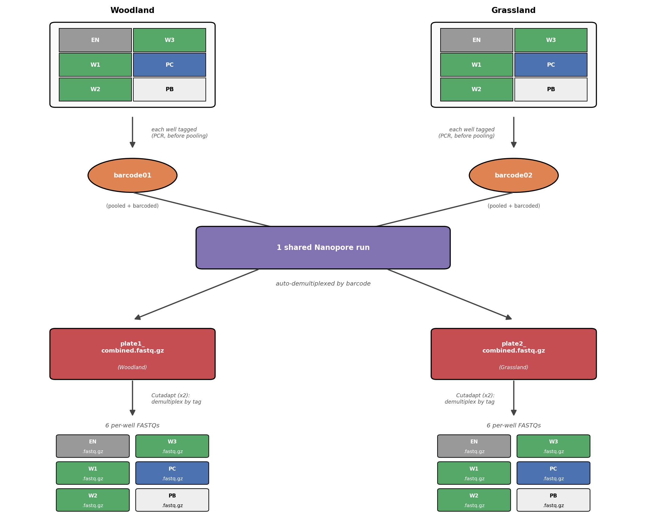
Barcoded DNA from all wasps and both sites were pooled together onto a single, shared sequencing run. Each site gets its own Nanopore barcode (a run-level ID, resolved automatically by the sequencer) — and within each site, individual wasps and controls are told apart by tags (a finer-grained ID, resolved by the pipeline itself). You’ll build the exact plate layout, samplesheet, and metadata for this scenario yourself in Steps 2–3, then run the pipeline for real in Step 4 using the small dummy dataset.
Step 0 — Pipeline overview
Before diving in, here’s the whole journey from raw reads to results in one picture — every stage you’ll actually see running in Step 4:

- Raw Nanopore reads (one FASTQ per plate, already split by barcode)
- NanoFilt → filter reads by length/quality
- NanoPlot → QC report, before and after filtering, and after demultiplexing
- Cutadapt (×2) → demultiplex by forward tag, then reverse tag → one file per well
- amplicon_sorter → cluster each well’s reads into consensus sequence(s)
- Medaka → polish each consensus
- BLAST → search each consensus against your reference database
- taxonomizr → assign taxonomy from the best BLAST hit
📚 Good background resources
- Nanopore sequencing — how it works (Oxford Nanopore)
- Cutadapt documentation — the demultiplexing tool this pipeline uses
Step 1 — Inspect the raw data and pipeline requirements
The pipeline ships with a small built-in test dataset, but we will use a custom one made for this training, following the case study above. Clone the pipeline repository first:
git clone https://github.com/Eco-Flow/nanoporemetabarcoding.git
cd nanoporemetabarcoding
What is git clone? git clone downloads a full copy of a repository from GitHub (or another code host) onto your machine. You’ll usually need this step to run a pipeline that isn’t on nf-core — nf-core pipelines can be run directly by name (nextflow run nf-core/...), since Nextflow fetches them for you automatically.
The raw reads live in wasp_course_data/. Nanopore FASTQs are gzipped, so peek at them with zcat:
▶️ Try it — peek at a raw FASTQ
zcat wasp_course_data/barcode01/plate1_combined.fastq.gz | head -8
✅ Expected output
Groups of four lines per read, same FASTQ format as Illumina — but unlike the paired, fixed-length RNA-Seq reads from Part 3, Nanopore reads are single, variable-length long reads with no pair:
@<read id> ...
ATGCGT...(a few hundred bp, length varies read to read)
+
!%'&&$#"...(quality string, same length as the sequence)
▶️ Try it — count the reads
zcat wasp_course_data/barcode01/plate1_combined.fastq.gz | wc -lFASTQ uses 4 lines per read, so divide the line count by 4 to get the number of reads. This file is deliberately tiny (a handful of reads per well) so the whole pipeline runs in minutes.
Also inspect the other files you’ll need:
cat wasp_course_data/tag-primer_f.fasta      # forward tag-primer sequences
cat wasp_course_data/tag-primer_r.fasta      # reverse tag-primer sequences
cat wasp_course_data/metadata.csv         # which tag combination = which sample
Now that you’ve seen the files, check the pipeline’s own usage on its GitHub page — README.md — to see how they map to actual inputs.
To run nanoporemetabarcoding you need:
- a samplesheet (
--input) — one row per FASTQ. For this experiment, every FASTQ represents one Nanopore barcode/plate - (optional) a metadata sheet (
--metadata) — one row per well, mapping a forward+reverse tag-primer combination to a sample name. Without it, wells are reported under their raw tag-primer combination instead of a human-readable sample name — worth having for any experiment with more than a couple of wells per plate - a forward tag-primer FASTA (
--tags_f) and a reverse tag-primer FASTA (--tags_r). This are needed for demultiplexing - a reference database for taxonomy — either
--blast_db(pre-built) or--custom_db(a FASTA the pipeline will build a BLAST DB from). For this workshop we are going to use a custom one, as a BLAST database can be hundreads of gigabytes in size - a taxonomy ID database (
--sql_db) — a separatetaxonomizrSQLite file that maps each BLAST hit’s accession to its full taxonomic lineage (domain → species).--custom_db/--blast_dbonly supply the sequences to search against; this is what turns the winning accession into an actual species name afterward
Step 2 — Design a samplesheet
The samplesheet links each FASTQ to an ID. It has just two columns:
| Column | Meaning |
|---|---|
id |
An identifier you choose for the FASTQ (can be anyrhing, but cannot contain spaces or ‘_’) |
fastq |
Path to that ID’s single, merged FASTQ file |
▶️ Try it — design
samplesheet.csvfor the wasp experiment Using the table in The experiment (2 sites → 2 plates → 2 barcodes), write out what the samplesheet should look like.
Cheat sheet — samplesheet.csv for the wasp scenario
id,fastq
woodland,wasp_course_data/barcode01/plate1_combined.fastq.gz
grassland,wasp_course_data/barcode02/plate2_combined.fastq.gz
One row per ONT barcode/plate. fastq must point to a single, existing .fastq.gz file — if your sequencer produced several chunk files per barcode, merge them (e.g. cat) before writing the samplesheet.
Step 3 — tag-primer FASTAs and metadata
First, what a tag-primer FASTA actually is: a regular FASTA file where:
- the header is a short label for that sequence (in the case of this study, it’s a combination of the tag and the primer’s original tables, but it can be anything).
- the sequence is the tag fused to the primer — the exact DNA Cutadapt searches for and trims off each read during demultiplexing (Step 0)
You need two: one for the forward tags (--tags_f) and one for the reverse tags (--tags_r). A read matching one entry from each file, forward and reverse, is what identifies which well it came from.
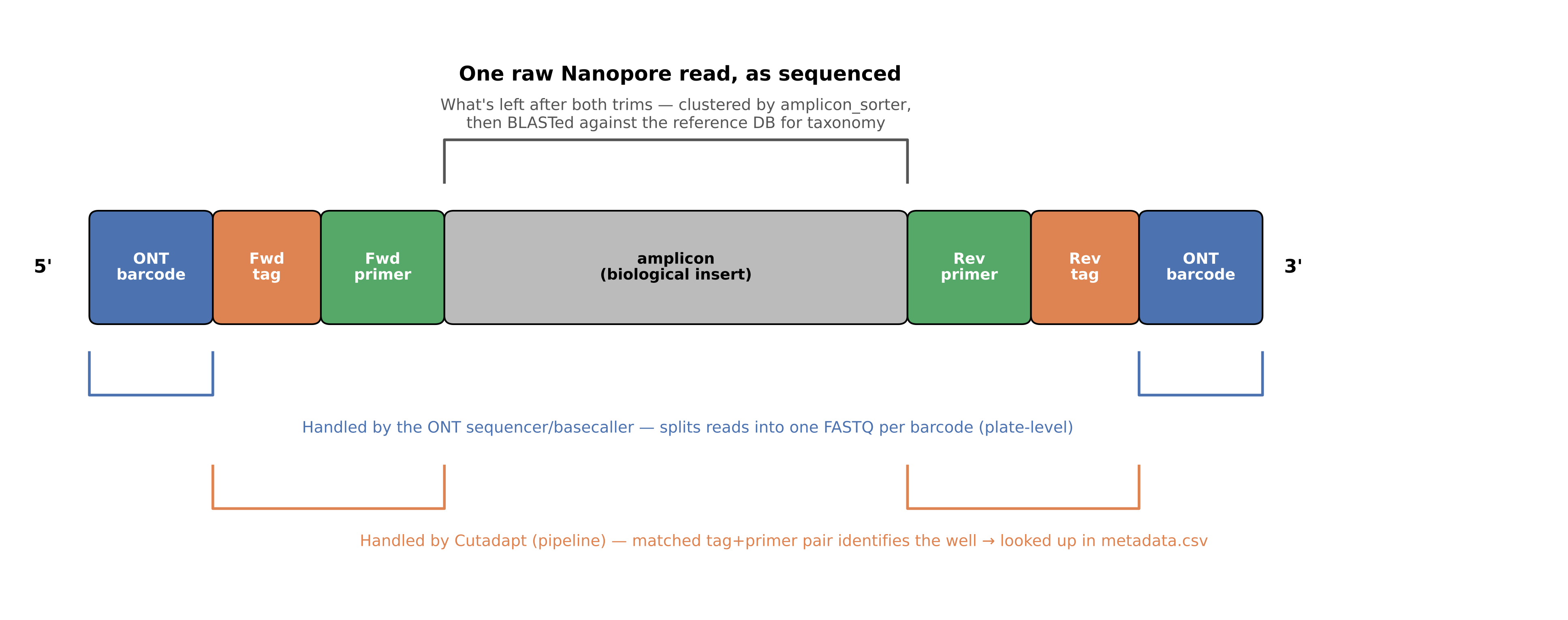
The metadata sheet is optional — but it’s what resolves each demultiplexed well down to a sample name; skip it and the pipeline reports each well under its raw tag-primer combination instead. You build it by mapping every tag-primer combination (using the same FASTA headers from above) to the sample it belongs to. It has three columns:
| Column | Meaning |
|---|---|
id |
Must match a plate id from the samplesheet |
tag-primer_comb |
<forward tag header>_<reverse tag header> — must exactly match headers in your tag-primer_f/tag-primer_r FASTAs, and every combination must be separated by a _ |
sample |
The name you want in the final ASV table — must be unique within each plate |
⚠️ Key rule:
tag-primer_combis a straight string match against your FASTA headers. If the tag names don’t match exactly (typos, case, extra characters), that well’s reads won’t be assigned to a sample.
▶️ Try it — design the metadata for the woodland plate
The woodland plate has 3 forward tags (
F1_WaspExF_Tab1,F2_WaspExF_Tab2,F3_WaspExF_Tab3) and 2 reverse tags (R1_LuthienR_Tab29,R2_LuthienR_Tab54), giving 6 wells: one extraction blank, one positive control, one PCR blank, and 3 adult wasps netted in the Woodland site. Write out the FASTAs and the metadata rows.
Cheat sheet — tag-primer_f.fasta / tag-primer_r.fasta
>F1_WaspExF_Tab1
AACAAGCCCCTTTATCWTSWRRWWTTGS
>F2_WaspExF_Tab2
GGAATGAGTCCTTTATCWTSWRRWWTTGS
>F3_WaspExF_Tab3
AATTGCCGGTCCTTTATCWTSWRRWWTTGS
>R1_LuthienR_Tab29
GAGTAACCACTTCWGGRTGWCCAAARAAYCA
>R2_LuthienR_Tab54
CGATGAGTTACTTCWGGRTGWCCAAARAAYCA
Cheat sheet — metadata.csv for the woodland plate
id,primer_comb,sample
woodland,F1_WaspExF_Tab1_R1_LuthienR_Tab29,EXT_NEG_F1_R1
woodland,F2_WaspExF_Tab2_R1_LuthienR_Tab29,WD_wasp01
woodland,F3_WaspExF_Tab3_R1_LuthienR_Tab29,WD_wasp02
woodland,F1_WaspExF_Tab1_R2_LuthienR_Tab54,WD_wasp03
woodland,F2_WaspExF_Tab2_R2_LuthienR_Tab54,POS_CON_F2_R2
woodland,F3_WaspExF_Tab3_R2_LuthienR_Tab54,BLANK_F3_R2
Same mapping, laid out as a plate layout:
woodland plate (barcode01)
| | R1_LuthienR_Tab29 | R2_LuthienR_Tab54 |
| — | — | — |
| F1_WaspExF_Tab1 | EXT_NEG_F1_R1 (extraction blank) | WD_wasp03 |
| F2_WaspExF_Tab2 | WD_wasp01 | POS_CON_F2_R2 (positive control) |
| F3_WaspExF_Tab3 | WD_wasp02 | BLANK_F3_R2 (PCR blank) |
▶️ Try it — design the metadata for the grassland plate
The grassland plate reuses the same forward/reverse tag scheme as the woodland plate (the same primer plate design was run at both sites), so you already have every header ID you need — no need to open the FASTA files again. Work straight from the plate layout below: the row/column labels give you the tag headers, and each cell gives you the sample that goes with that combination.
grassland plate (
barcode02)
R1_LuthienR_Tab29R2_LuthienR_Tab54F1_WaspExF_Tab1EXT_NEG_F1_R1(extraction blank)MW_wasp03F2_WaspExF_Tab2MW_wasp01POS_CON_F2_R2(positive control)F3_WaspExF_Tab3MW_wasp02BLANK_F3_R2(PCR blank)
Cheat sheet — metadata.csv for the grassland plate
id,primer_comb,sample
grassland,F1_WaspExF_Tab1_R1_LuthienR_Tab29,EXT_NEG_F1_R1
grassland,F2_WaspExF_Tab2_R1_LuthienR_Tab29,MW_wasp01
grassland,F3_WaspExF_Tab3_R1_LuthienR_Tab29,MW_wasp02
grassland,F1_WaspExF_Tab1_R2_LuthienR_Tab54,MW_wasp03
grassland,F2_WaspExF_Tab2_R2_LuthienR_Tab54,POS_CON_F2_R2
grassland,F3_WaspExF_Tab3_R2_LuthienR_Tab54,BLANK_F3_R2
💡 Always include controls.
EXT_NEG(extraction blank — no tissue),POS_CON(mock DNA of a known reference species), andBLANK(PCR no-template control) are how you catch contamination and confirm the assay worked — track them through the metadata sheet exactly like a real sample.
Step 4 — Run the pipeline
Now put the theory aside and actually run the pipeline:
Read the parameters block in nextflow.config for the full option list.
Cheat sheet — the full command
nextflow run main.nf \
-profile docker \
--input wasp_course_data/samplesheet.csv \
--metadata wasp_course_data/metadata.csv \
--tags_f wasp_course_data/tag-primer_f.fasta \
--tags_r wasp_course_data/tag-primer_r.fasta \
--custom_db wasp_course_data/custom_db.fasta \
--sql_db wasp_course_data/nameNode.small.sqlite \
--outdir results
👉 Single vs double dashes matter! A single dash (
-profile,-resume) is a Nextflow core option. A double dash (--input,--metadata,--outdir) is a pipeline parameter defined by nanoporemetabarcoding.
✅ What success looks like: Nextflow prints a banner, then a live list of processes as they run (
NANOFILT,NANOPLOT,CUTADAPT×2,AMPLICON_SORTER,MEDAKA,BLAST_BLASTN,ASSIGN_TAXA, …). On the tiny test data this should complete in a few minutes, plus a bit longer the first time while Docker pulls the containers.
Troubleshooting Step 4
❌ Missing required parameter: --input / --outdir
Check every --input, --metadata, --tags_f, --tags_r and --outdir is present and spelled correctly.
❌ A well/sample is missing from the final ASV table
Almost always a primer_comb mismatch — the tag combination in metadata.csv doesn’t exactly match <tags_f header>_<tags_r header>. Double-check spelling and case.
❌ .command.sh: ... command not found (exit status 127)
You forgot -profile docker. Without it, Nextflow expects every tool (Cutadapt, Medaka, BLAST, …) to already be installed locally.
🔍 Debugging any failure — the same recipe as before. Every task runs in its own directory under
work/, named after the hash Nextflow prints ([a1/b2c3]). When a task fails, Nextflow prints aWork dir:path —cdinto it and read.command.err(the error),.command.log(all output) and.command.sh(the exact command that ran). Remember to usels -a, since those files are hidden. This is covered in full in RNA-Seq · Step 6 — Monitoring a run.
Step 5 — Explore the results
Once you see Pipeline completed successfully, look inside results/:
ls results
✅ Roughly what you'll see
nanoplot/ blast/ assign_taxa/ community_matrix/ plots/ multiqc/ pipeline_info/ reads_per_step/
Where to look, in order:
multiqc/multiqc_report.html— one HTML report summarising QC across all samples (built from NanoStat).nanoplot/demultiplexed/<plate>/— per-plate read-length/quality plots, generated after demultiplexing, so you can sanity-check each well individually.reads_per_step/reads_per_step.csv— a read-count funnel: how many reads survived filtering, then each demultiplexing step. This is the fastest way to spot a well that dropped to zero reads (usually aprimer_combtypo).blast/<plate>.txt— raw BLAST hits for every consensus sequence.assign_taxa/<plate>/ASV_table_final.csv— the key output: one row per ASV (consensus sequence) per well, with its assigned taxonomy from the best BLAST hit.plots/proportion/*.png— stacked bar plots of taxonomic composition per barcode, at each rank listed in--tax_list.
🧬 If you completed Step 3: open
assign_taxa/.../ASV_table_final.csvand check whetherEXT_NEGandBLANKpicked up any real hits — if they did, that’s contamination worth flagging, exactly as it would be in a real run.
Step 6 — Running on an HPC (Myriad example)
🎯 For the general concepts see Part 8 · Running a pipeline on an HPC (getting a pipeline, submitting and watching jobs, keeping Nextflow alive) and, if your cluster has no config yet, ★ Advanced: setting up Nextflow for your HPC (talking to your HPC admin, writing a config from scratch, testing it). This step is a concrete worked example on top of those, using UCL’s Myriad cluster.
Because nanoporemetabarcoding was build from the nf-core template, it inherits nf-core’s institutional config mechanism — so if your institution already has a config, you don’t write anything yourself. Browse nf-co.re/configs to check — UCL’s Myriad cluster is listed there.
⚠️ Before you run anything, follow the setup steps on your cluster’s own config page — e.g. for Myriad that’s nf-co.re/configs/ucl_myriad. Each institution’s page documents cluster-specific prerequisites — for Myriad that means loading a specific Java module (
module load java/temurin-17/17.0.2_8, added to your.bashrc) and installing Nextflow itself into your own~/bin/, since it’s not preinstalled.
nextflow run main.nf -profile test_synth,ucl_myriad --outdir results -resume -bg -w ./Scratch > log
Myriad’s cluster uses singulairty to manage dependecines. You can use conda instead if singulairty is not installed in your HPC.
👉
-wsets Nextflow’s work directory (defaults to./work) — where every task’s intermediate files are staged, and what both Nextflow’s caching and-resume(Step 7) rely on: delete or move it, and there’s nothing left to resume from. On an HPC it’s worth choosing this deliberately before a real run, since these files can get large fast — point it at your cluster’s scratch space rather than your home directory, to avoid filling shared storage.
💡 What is Singularity? Docker needs a background daemon running with root privileges — not something shared HPC systems can safely allow every user to have. Singularity (Apptainer is another equivalent option) is a container engine built for exactly this situation: it runs the same kind of containers as Docker, but as your own user account, with no daemon and no elevated privileges required. That’s why HPC configs use
-profile singularityinstead of-profile docker— it’s not a style choice, it’s usually the only container engine installed in most cluster.
-profile ucl_myriad downloads and applies ucl_myriad.config automatically — no -c flag, and no separate -profile singularity needed (the profile enables Singularity itself). It’s worth reading the actual config to see what a real one looks like:
What's actually in ucl_myriad.config
executor {
    name = 'sge'
    queueSize = 100
    submitRateLimit = '10/1s'
}

process {
    penv = 'smp'
    clusterOptions = {
        def mem = task.memory.mega
        def cpus = task.cpus
        def memoryPerCpu = mem/cpus
        "-S /bin/bash -l mem=${memoryPerCpu}M "
    }
}

singularity {
    enabled  = true
    cacheDir = "${System.getenv('HOME')}/Scratch/.apptainer/pull"
}
Two things worth noticing, since they’re easy to get wrong writing your own config:
- Myriad uses SGE, whose
-l mem=flag is memory per core, not per job — so the config computestask.memory / task.cpuson the fly for every process, rather than using a single fixed value. - The Singularity cache (
cacheDir) is pointed at~/Scratch, not the home directory — home quotas on Myriad are small, and containers are large. Always check where your own cluster wants large/scratch data to live (Step 1 in hpc_config.md). This is usally the case for most HPCs.
▶️ Try it — test the config before a real run
nextflow run main.nf -profile test_synth,my_hpc_config --outdir resultsSame idea as Step 6 of hpc_config.md: run the tiny test profile first and check the banner says
executor > sge, notexecutor > local— that confirms jobs are actually going to the scheduler, not running on the login node.
While jobs are running, watch them with qstat on SGE — the SGE equivalent of Slurm’s squeue (both are covered in Part 8). Both print a status column whose codes mean the same underlying thing but look different:
| Meaning | qstat (SGE/Myriad) |
squeue (Slurm) |
|---|---|---|
| Running | r |
R |
| Queued, waiting for resources | qw |
PD |
| Held (won’t start — e.g. a dependency isn’t met) | hqw |
PD (reason shown separately, e.g. Dependency) |
| Finishing up / cleaning after the job ends | t (transferring) |
CG (completing) |
| Completed successfully | (drops off qstat entirely — check with qacct -j <jobid>) |
CD, briefly, then drops — check history with sacct -j <jobid> |
| Failed to start (config/resource error) | Eqw |
F |
| Hit its time limit | (job is killed; check qacct -j <jobid>) |
TO |
| Suspended | s / S |
S |
| Being cancelled/deleted | dr / dt |
CA |
🔍
Eqwis the one you’ll actually hit while debugging a config. It means the job was rejected before it even started — almost always a badclusterOptions/penv/queue name. Runqstat -j <jobid>(SGE) orscontrol show job <jobid>(Slurm) to see why it was rejected, rather than just that it was.
💡 Other schedulers (Slurm, etc.): the same institutional-profile trick applies wherever nf-core/configs has a listed cluster — check https://nf-co.re/configs first. If yours isn’t listed, hpc_config.md has side-by-side minimal config examples for both SGE and Slurm: the main differences are
executor.name('sge'vs'slurm'), how you request memory (SGE: per-core viaclusterOptions; Slurm: per-job via--mem), and the queue/partition option name. A Slurm submission script for this same pipeline would look like the Slurm driver-job example in Part 8, swapping in nanoporemetabarcoding’s--input/--metadata/--tags_f/--tags_r/--custom_dbflags shown above.
🙋 No institutional config for your cluster? Just get your HPC admin in touch with us at Eco-Flow and we will build one.
Step 7 — Resuming a run and changing options
Changing an option
Taxonomy assignment has adjustable identity thresholds per rank — e.g. --spident (species), --gpident (genus). Work out how you’d tighten the species-level threshold to 98% identity, but don’t run it yet:
Answer — the modified command
nextflow run main.nf \
-profile test,docker \
--outdir my_results \
--spident 98
The -resume flag
Add -resume and Nextflow reuses cached results for any step whose inputs haven’t changed — so re-running the command above only re-executes taxonomy assignment (and anything downstream of it), not the demultiplexing or clustering steps.
✅ What you’ll see with
-resume: unchanged processes markedcached, e.g.[a1/b2c3] ...:CUTADAPT_FORWARD (woodland) [100%] 1 of 1, cached: 1 ✔.
Finish
🎉 You’ve finished this practical. You’ve gone from raw Nanopore reads to a taxonomically-annotated, per-sample ASV table and community matrix — and designed a samplesheet/metadata scheme for a real multi-plate, primer-tagged experiment.
Next steps:
- Adapt what you designed in Steps 2–3 to your own primer-tag scheme and run it on your own data.
- Explore the full parameter list in
nextflow.config— worth tuning per-rank identity thresholds (--spident/--gpident/--fpident/--opident) and--tax_listfor your own taxonomic group. - Running on a cluster other than Myriad? Step 6 above covers the concrete example; Part 8 · Running a pipeline on an HPC covers the general concepts (including Slurm and SGE examples), and ★ Advanced: setting up Nextflow for your HPC covers writing a config if your cluster doesn’t have one.